Big G equals six point sixty seven times ten to the negative eleven

And Here it is. The final activity. Hoboy!

---

Bruh. This is a Physics subject right?
Umm yeah?
Well. You know... After ten activities in one semester I've been wondering. Where's the Physics?
But $SCIENCE$...
Yeah. You've been saying science this, science that. But I just don't feel like I've seen any Physics stuff.
N-n-n-NANI!?

Well fine. Let's do something Physicsy. Choosy >&↑^%#+}~@%#.
Uck don't you mean PRINCESS. Cuz I'm like super fabulous. Ewl

---

Back in first year high school, on the second week of classes, my EarthSci (ence) teacher asked us to find the value of the oh so mighty big $G$.
That's the universal gravitational constant you pleb. The meeting after he told us that we should memorize this... $BY \, HEART$. And so I did.
Yeah It's one of those things I'll never forget.

$G = 6.67 \times 10^{-11} N \frac{m^2}{kg^2}$

Big GEE equals six point sixty seven tayms ten to the negative eleven newton meter squared over kilo gram squared.

The following year our Physics 1 teacher happened to be the same person. This time around he made us memorize three equations $by \, heart$.
These are, in his words, "equations according to our friend Isaac." And so right there on my "beautiful notebook" which was checked and graded every quarter, lies three beautiful equations inside red boxes shaded with yellow.

These three equations state

These are the equations for velocity, force, and free fall motion from rest.
I'd show you my 2008 notebook if I my "memories box" did not "inexplicably" disappeared after my brother cleaned the room.

---

Yes! We are going to do free fall. Ahh what best to relate to Physics than the kinematics of freely falling bodies.
Specifically we will determine the acceleration due to gravity on Earth.

Let's do this!
We took a video of a falling tennis ball.
The ball was dropped from a height of 150cm which lasted for about three seconds. This already included a few bounces. Because as the third beautiful equation suggests, a free falling body only needs about 0.55s to travel 150cm from rest.
The video was supposedly shot at 60 frames per second. I only used the frames from when the ball reached maximum height after the first bounce until it reaches the bottom of the camera view.

I did not use the first falling part because by the time the ball enters the camera range it is too fast that it exists in fewer frames.
Also as Roland Romero so eloquently puts it, the ball near the bottom goes $Bvvffffff$

Dahell is "Bvvffffff"?
Oh you know. A cat goes "meow." A chicken goes "bok bok bok." A cow goes "mooooo."
And 'a comet goes "$Bvvffffff$"' - Romero(2016)

For those who don't understand idiot language it means that the ball is producing after images.

Anyway. To track the motion of the ball, I first segmented the image. Remember Activity 7? Yeah that. Here I used parametric segmentation using gaussian pdf and the whole ball as the region of interest. Somehow I could not get the non-parametric method to work here.
Here's how it looks.

Due to bad lighting and motion blur, the extracted ROI sometimes (more like often) have holes in it.
Now this is not really an issue as long as there's not too much holes, or the holes are radially symmetric with respect to the center of the ball.
Why? Because we will be using Blob Analysis to find the center of the ball.
As long as the calculated centroid is not too far from the center of the ball we are fine.

The red dot signifies the position of the calculated centroid. We can observe that it is indeed not too far off from the center.

Now let's plot the position of that centroid with respect to time

Looks quadratic. It could be right.

How exactly do we get the acceleration?
Well what if we plot $y$ vs $t^2$. Since $y = 1/2 at^2$, the slope of this plot is going to be $a/2$.

The slope of this plot is $381 \rm{px} /324 \rm{frames}^2$ or $a = 2.35 \rm{px} /\rm{frames}^2$
Now lets do some conversions. The white board background has a width of 80cm or 650 pixels. We also know that the video is shot at 60 fps.
Hence: $1 \rm{px} = 0.0012 \rm{m}$ and $1 \rm{frame}^2 = 1/3600 \rm{s}^2 = 0.00028 \rm{s}^2$

So our final measurement for the acceleration due to gravity is $10.07 \rm{m/s^2}$ which has a 2.8% deviation from the accepted value $9.8 \rm{m/s^2}$

---

Aaaand that's the last activity. Good job me. Good job.
I will give myself one last solid $10/10!$
$GG \, EZ$

I would like to acknowledge Anthony Fox and Roland Romero as my groupmates in the data gathering of this experiment.
Special thanks to Kit Guial for the extraction of frames from the video.
Shout out to my favorite high school teacher who made me want to take a Physics course, Mr. Delfin C. Angeles.

Weird thanks to my blog's second voice. My imaginary fan. Yey.
Uck Puh Lease. Call me PRINCESS. Like ew. This is so embarassing. Oh my Gawsh. Ewl. Like whatever. Se ya... neva.


A very special thanks to Dr. Maricor Soriano for a wonderful semester and for all the lessons I have learned.
:D


- Bear In The Big Blue House - Goodbye Song
Bye Now.

Activity X - Menipulation of histogram

Activity $Tenenene \, nene \quad Tenenene \, nenen$
I will really die alone now.

---

Pictures are a technological marvel. They show you things as they were. They are infallible reconstructions of what was. OR SO THEY WANT US TO BELIEVE!

Do not be fooled. Pictures are lying bad boys. Everything they show is real, true but we can still easily be fooled. It is all about framing and lighting. By showing us some parts and hiding others behind the shadow, we arrive at the wrong conclusion.
Ahem media ahem

It is time to rise against the pictures!
Wha...?
It is time to shed light to the truth. To bring the real issues out of the shadows!
Like seriously what?

These lying pieces of PICS, have been hiding information from us all along. And we will need the power of Dr. Soriano's SEA-men.
(I feel a 5.0 coming)
You're lucky if you don't get disciplinary action broh.

---

Dahell? Who wrote the previous section... Definitely not me! Anyway...

Look at this picture of Dr. Soriano's team in action at the sea.
Bruh!

Look at that nice lady to the left. Can you see anything behind her?
Umm no...? Uhh maybe... I kinda umm... I don't know
What about the guy in blue. Is his right foot also wearing slippers?
Uhh it kinda looks like it but... uhh I'm not sure broh.
Exactly.

Now look at this

Holy mama. Where'd those lines come from? Wait whut, her shirt had wrinkles? I did not notice that. And yup that guy is totally wearing slippers on both feet. Ha... How?

Well my friend this is a simple case of
Science?
No! Stop interrupting me...
$SCIE...$ uhh.. i mean $HISTOGRAM \, MANIPULATION$

This is how it works.
For simplicity let's do it in grayscale.

First we get the histogram (pdf) of the grayscale values. It will look like this.

Then we get the cumulative distribution function (cdf). Like so.

See that sharp increase at the end suggest that some of the brighter features are highlighted while others are downplayed. 

So here's what we're gonna do. We're gonna think of an "ideal" version of the cdf. And then we're gonna force our image to conform. 

Histogram manipulation for idiots.

1. Get cdf of image

For each pixel in the image:

  2. Get cdf value of pixel

  3. Match to cdf value in desired cdf

  4. Take the corresponding pixel value of that that cdf value

This image illustrates what's happening

Remember that "improved image" before. I used a Gaussian cdf for that.

Here's a few more results using Gaussian cdf's with different standard deviation values.

Actually, the best looking improvement I got was using a uniform pdf. Or well that's going to look like a linear cdf. 

Yes treat all information equally!

This is how it looks like using a linear cdf (uniform pdf)

$GREAT$

Of course we all know what the next step is. COLORED!

To make things easier, we are gonna convert the image into rg chromaticity coordinates.

I'm not gonna explain that here. Go back to activity 7 :)

Basically we do the same thing we did for the grayscale image on the Intensity or I channel of the rgI converted image. Then we simply put it back on the RGB color space for rendering. $EZ$

 $TENEN$

 And there it is, again using linear cdf. Now we can see more features and the color does not seem way off. Horay!

Uhh lets put them side by side for comparison

Original (left) and Linear cdf reconstruction (right)

Good, good.

Let me just put it here because I can.

Before and after linear cdf reconstruction of a "bright" scene

Wow I can totally see the some of the lightbulb case pattern.

Yeahp. $GG$

---

Hohoho that's over with.
Of course histogram manipulation is far from the results of using High Dynamic Range imaging. Using HDR is going to show a lot more features but requires a multiple pictures of a scene under different exposures. Histogram manipulation needs just that one and can totally be used on those 'noob' pictures in your collection.

Good job me.
Hmm not bad. Not bad at all. 
For this I give myself a solid...
Ten!
What? 
10/10! That's right. Look at me. I give the grades now.

Special Thanks to Dr. Maricor Soriano and her team for the image.

Morphing DNA Causes Cancer

Now we're gonna learn about the mighty morphological operations.
These are operations that perform certain transformations to images, usually by adding or removing pixels.

For the sake of this activity we will only deal with binary black and white images.
The most important part in applying morphological operations is the Structure or Structuring Element (SE). This is a template of sorts that we will use to perform the transformations.

The basic morphological operations are the $DILATION$ and $EROSION$.
In Dilation, we survey all pixels in the image. We will impose the the reflection of the structuring element on each of these pixels. If the "whites" of the imposed SE encounters a "white" pixel in the image, the pixel where the SE is imposed turns white, potentially adding more white pixels in the image.

In set notation, the dilation of image A by SE B is
$A \oplus B = \{ z|(\hat{B})_z \cap A \neq \emptyset \}$

In Erosion, we impose the structure element on all the white pixels. If any of the whites of the imposed SE encounters a black pixel in the image, the pixel where the SE is imposed turns black.

In set notation the erosion of image A by SE B is
$A \ominus B = \{ z| B_z \subseteq A \}$

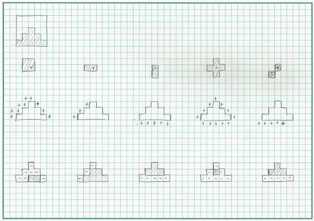
Here are some examples of how Dilation and Erosion works
In the following pictures, the first row show the original image.
The second row shows the structuring element. The third and fourth shows what happens after Dilation and Erosion respectively.

Boxes with hash represent white pixels.
Blue plus (+) signs show white pixels to be added after dilation
Red minus (-) signs show white pixels to be turned black after erosion

Yes I know this was supposed to be a triangle with 4px base and 3px height but I don't know how to draw that properly so here's a triangle with 5px base.

And this one has a weird configuration due to space limitations

Bro that looks messy. Can you computerize that.
In time my friend... in time.

---

Well... adding and subtracting white dots doesn't seem useful now does it?
That's because you don't know $SCIENCE$
Stop saying "science" like it's a magic word, you're giving me cancer.
Well why don't we take tissue samples from you and check if you got cancer.
Wha... What?
Oh yeah. With the power of morphological operations we are going to identify cancer cells. Because ...
Let me guess. Science?
$SCIENCE!$

Now here is a bunch of circles. Yep those are cells, normal-looking cells. Believe me they are.

But where? It's all gray and stuff.
Remember image segmentation? Well... $BOOM \, SEGMENTED$

El Oh El. You like totally feyald. Ewl. Noowb
That's the limit of segmenting by threshold. Now behold the power of...
Science?
Wha? No. $MORPHOLOGICAL \, OPERATIONS$
Specifically we will use the OPEN operation. This is defined as an Erosion followed by a Dilation.
Why?
Because, using Erosion we can remove the smaller "noise"-like pixels blobs. Then by using Dilation, we can restore-ish the bigger blobs to their original form. All right let's do this.

$Krakabooom$

Behold the power of $OPEN$ operation

This is done by using a 10px circular SE

Okay now what?

Now we can find the size of normal cells. Here's the pdf broh.

$\mu = 695$ $sigma = 521$

Wha? 521 standard dev?

I dunno man. That's what Scilab gave me.

Well whatever. From this I determined that normal sized cells have an area of about 550-750 pixels. 

Determined? More like declared so.

Yeah yeah whatever.  

Anyway. Here is the picture of your cells. YES THEY ARE.

$YES...THEY...ARE$

We expect that cancer cells are bigger than ordinary cells. Because they are greedy as $\mathcal{F} \cup \subset \prec$

Using our might morphological operations the sample is segmented. And then $BANG$ by the power of FilterBySize, I isolated the odd-sized blobs. And viola.

 

$BOOM \, YOU \, HAVE \, CANCER$

Yeahp you got 5 cancer cells alright.
Bu...
$SCIENCE$

---

Mehehehe again I'm setting my standards low here.
For a Mission accomplished, I'm giving myself a 10/10!
No no, your dilation/erosion sucks
Fine, I'm giving myself a $9/10$ 

Special thanks to this German(?) guy for explaining-ish dilation and erosion
And thanks to Mr. Kit Guial for pointing out that video

Do Re Mi Fa Sci Lab

Ohhh Activity 9....
This is uhh. hmm
This activity took me quite a long time. But this post is going to be very short.

I really worked hard on another piece of music...
Oh right ugh...
In this activity we're gonna make Scilab play us music by processing the image of a music sheet.
So anyway as I was saying. There was this quite complicated music sheet that is very special to me. I really wanted to use that. In fact I spent the long weekend before November 2 devoted to that and make a pun about how I poured all of my soul into this activity in celebration of All Souls Day and stuff.

Unfortunately for me, I did not get the piece playing quite right. And no, I'm not willing to post that half baked result. I mean sure I do like the output of that one (I got LSS quite a few times because of it) but, as I said that music piece is special to me so I just can't bring myself to post it until it's perfect. I plan to finish that during this Christmas break so yeah... stay tuned.

This is now all just for the sake of completion.

Suppose we have a piece of sheet music. For simplicity I will only show three 3/4 measures.

Step 1. Binarize the image

Since I binarized this in MS Paint, some features are lost. Thankfully, those missing features are supposed to be removed later on anyway.

Step 2. Remove staff and "flagpoles" (those things that attach notes to their flags)
Using morphological operations (see Activity 8)
I Dilated the image using a thin horizontal line. Thus removing the flagpoles (and all black features that are thin horizontally)

Then I Dilated the image again, now using a thing vertical line. Thus removing the staves (and all vertically thin black features)

Step 3. Extract notes
Notes are in general (or always?) circular. I obtained the notes by using the OPEN operator using a circular Structure Element. Due to the nature of extraction, this step can be done right after Step 1 and the results will be the same.

Doesn't OPEN get rid of the black features?
Right. I opted to first take the complement of the image (reverse black and white) due to the nature of Blob Analysis that will be used in the next steps

Step 4. Get note positions

Using the Scilab IPD Toolbox function, SearchBlobs and AnalyzeBlobs, the centroid of the notes can easily be obtained. Based on the y-position it is easy to identify the pitch (frequency) of the note to be played. While based on the x-position, we can identify the order with which to play them.

Step 5. Consider the flags.

Now that we know the position of each note, we can scan for it's surroundings. Shown here in red is the window with which I scanned the environment of the note.

I know this example is weird because they are all eight notes anyway. By simply counting the amount of blobs within the windowed region, it is easy to identify if the note is a quarter note, eight note, or even a sixteenth note. Each flag becomes a separate blob since we removed the 'flagpole'

Well, enjoy the music.

Here is a "raw" rendition.



And this one is using both an ASDR envelope and some "harmonics" effect
  

---

Oh right. The music is L's Theme from Death Note.
Arranged by Olivia Jelks
Obtained from Musecore.com

Hmm I guess I could say Mission Accomplished once more.
That's a $10/10!$ for me then.

Eeeevil Segmentation

$HEYYYYY \, I'M \, BACK$
It's been a while since the last post.
Too... lazy... to... blog...

Now we're gonna do IMAGE SEGMENTATION (dun dun dun)
What's that?
I'm sure you have an idea what it is. But for the sake of being complete I will insult your intelligence a bit.
Image segmentation is the process of isolating a part of an image that contains information that we want, or in general just being interesting so to speak. Let's call that part the Region Of Interest (ROI) and the rest of the image becomes the background.

When the image is in grayscale (that's black and white you pleb), it is quite easy to separate certain features.
Take a look at this cheque for example. Yes CHEQUE. It looks sexier than it's Murrican spelling.

Now I want the grey background to be gone and only take the texty stuff.
What to do? BAM! THRESHOLDING.
I simply keep the black parts and make all "non black" pixels white.
Just like that? Yeahp. $EZ$

Here is how that cheque looks like in different thresholds from 50-250 by intervals of 25.
I know that you know by now that I like animated GIFs. And you probably do to. So here.

 

$Shablam$

Now let's be a bit more scientific than trial and error. 

dude TaE method is so scientific

Epepep. Shhhh shhhh. Let $SCIENCE$ happen. 

So we now take the histogram of the pixel values of the image.

 

$Histograaaaahm$

Well see that peak in the histogram? That's the background. $I \, think$. So basically everything above, say 160 pixel value is part of the background.

THRESHOOOOLD by 160 pixel value

 

$AMAZEBALSS$

Looks good brah. How'd you know to pick 160?

Trial and Error....

uhuh... what happened to "SCIENCE"?

Shut up.

---

Now what if it's colored?
Well we have two methods for that. The $PARAMETRIC$ and $NON-PARAMETRIC$ methods.
We'll get to that later.

Imagine SpongeBob. You probably imagined Patrick too right? Yeah because they are basically inseparable.

You and me forever in the underwater sun. Underwater sun~

But suppose that we really want to separate SpongeBob and Patrick.
Because we are
                       

So how do we do it?
Well first we have to understand the $rg \, CHROMATICITY \, SPACE$
This is also known as the normalized chromaticity coordinates (NCC), because we are normalizing the Red,Green, and Blue channels.

Here we separate the three channels of our colored image, R, G, and B.
Now we normalize them

$I = R+G+B$

$r = \frac{R}{I} \qquad g = \frac{G}{I} \qquad i=\frac{B}{I}$

The advantage of this is that we can now represent colors in just two dimensions $r$ and $g$.
The blue channel can easily be reproduced from the other two

$b = 1-r-g$

Here's how that chromaticity space looks like

 

https://en.wikipedia.org/wiki/Rg_chromaticity

Okay now what?
First we take sample of region of interest (ROI). Say Patrick's skin

 No no don't skin Patrick alive that's















I'm discussing here...


Anyway. From Patrick's skin sample we can now segment our image using two methods.
The first method is called parametric.
Why?
Because we assume a certain distribution of colors, say a Gaussian (Normal) distribution. $p(x) = \frac{1}{\sigma \sqrt{2\pi}} exp [-\frac{(x-\mu)^2}{2 \sigma^2}]$
Then we extract Parameters $\sigma$ and $\mu$ from our ROI sample.
 Actually we need two sets of parameters.
From the normalized red channel: $\sigma_r$, $\mu_r$
From the normalized green channel: $\sigma_g$, $\mu_g$
We use the extracted parameters to obtain the probabilities $p(r)$ and $p(g)$.
Now we multiply the two probabilities and call it $p(r,g)$.
This new probability tells us how likely a pixel in our image belongs to the same group as the ROI sample.

Here is what that combined probability looks like

 

After thresholding

Returning the color

Well we got a little bit of SpongeBob's tongue there. Can't be helped they're both pink

Hey I want a GIF.

Fine...

Soo about that other method?

Yes yes coming.

In the non parametric method, instead of assuming a distribution, we get the actual 2D histogram (pdf) of the ROI sample. Here's how that 2D histogram would look like.

In the rg color space it's gonna look like this

Bro that color space looks upside down

Yeah well that's just how Scilab plots.

Maybe in the future I'll try to fix that.

But for now $DEAL \, WITH \, IT$

So basically for whatever color exists in that histogram is part of our Region of Interest. So we go back to our image display only the colors that match our histogram.

Well I've taken so much space so here's your GIF

$SPLAKATOOM$

 Well compared to the parametric method, this one is a bit rough. The good thing is that it preserves a bit more features like Patrick's belly button, and SpongeBobs (tongue) cleavage.

---

Hehey we're done.
That's cool and all.
I'm not really aiming high here.
Cramming's bad mkay~

But I can say Mission Accomplished!
So I'm giving myself a full $10/10$ for this one.


Special thanks to:
Ms. Tisza Tronos' blog  for helping me work my problems in the non parametric method
Louie Rubio for pointing out that Scilab's windows can be merged like in Spyder wich makes me respect Scilab a bit more. And also for pointing out Ms. Trono's blog